Deconstructing Data Sketches
How 1,000 numbers can approximate millions of unique visitors in milliseconds

Recently I came across luminousmen article on Data Sketches. It explains how data sketches can replace expensive database count operations with quick approximations. The concept was very intriguing but confusing at the same time. So I spent some time diving into why it works. This article explains the same.
So what exactly is a Data Sketch and how does it help?
Just to recap the original article, imagine you are asked to find the unique number of users who visited a site today. You would ideally do a count distinct user query on the sessions table and it would workout fine, unless the number of events in the order of millions or billions. If thats the case your query would have to visit every record in the table to ensure it has the exact count of all unique users. This could either break the database or take forever depending on the table size and the compute being used. But we could use a data sketch and get an approximate count in under a second. How is that? For this we can use an analogy.
Imagine a large corporate like Walmart, who has millions of employees working each day. Now there’s an inspector who’s job is to find out how many employees checked in yesterday. Note that an employee could checkin in multiple times for different shifts, so his duplicate entry will not be counted. Now he can manually note down whenever an employee checks in for the day on his notebook. Whenever someone enters the office he could check his list if the person had already checked in for the day or not, and make an entry accordingly. This can work but it’ll be slow and tiresome. So he uses another method. One that gets an approximate count as he doesn’t need the exact number. He assigns each employee a unique tag when they check in. The tag could be any number between 1 to 4 billion (We need a large number space to avoid tag collisions). The rules are:
The number tag will be unique and exclusive to that employee
The number tag generator randomly picks a number from a UNIFORM distribution.
So when the employees start checking in, they are assigned different tags: 600, 11000, 565732, 573, 64968, 395345.. and so on from the space of 4,000,000,000.
What the inspector does, is that he keeps track of only the LOWEST K tags. Lets say its 1000. That is enough for him to get the approximate count of the employees who checked in for the day.
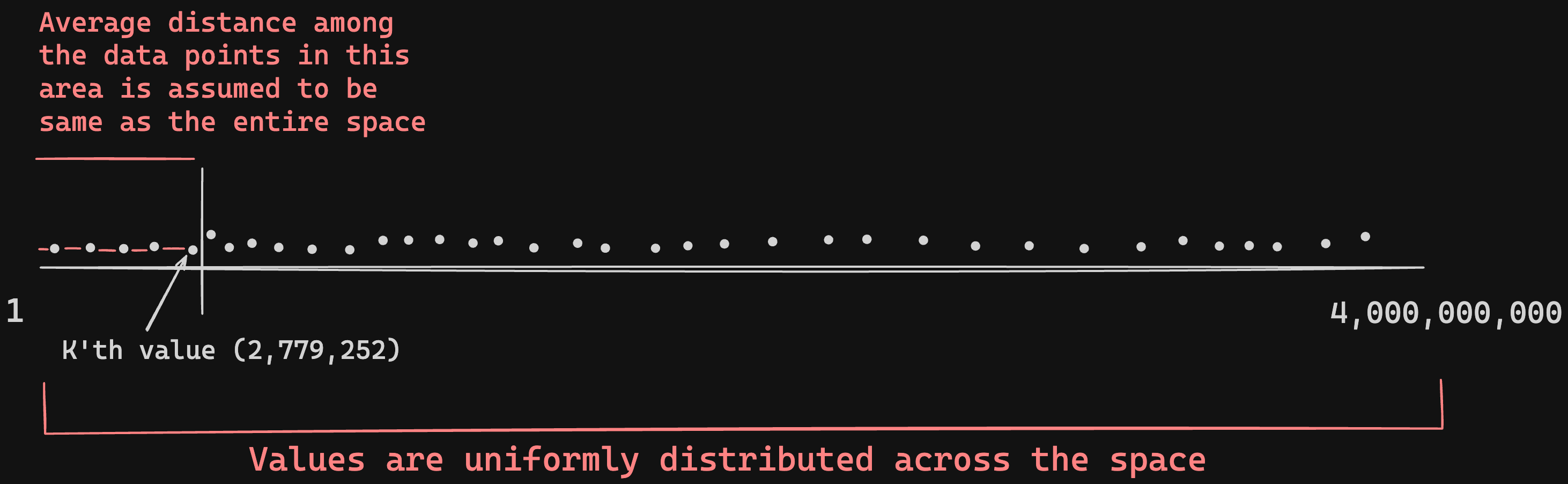
How does that happen?
Here’s the logic: Given that these tags are assigned in a uniform distribution, we can sort of assume that the gaps among all the tags are even. So what does that mean? It means that the gap between each number tag on a scale on 0 to 4 billion is around Total Space / Total tags. This also means that the gap between the first 1000 tags is the same as all the tags. i.e K’th tag / K. i.e V(K) / K.
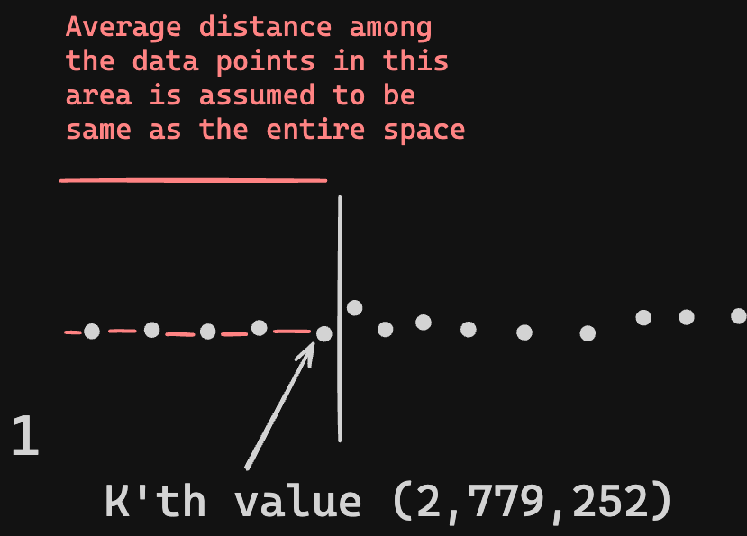
Does that make sense? If the 1000th lowest number tag is 2,779,252 then we do 2,779,252 / 1000 = 2779. That is the average assumed gap between tags. Now to get the total count, we just need to divide this gap with the total space. i.e 4,000,000,000 / 2779 = 1,439,366. This is the approximate count of all the unique tags, which is the unique number of employees who checked in today.
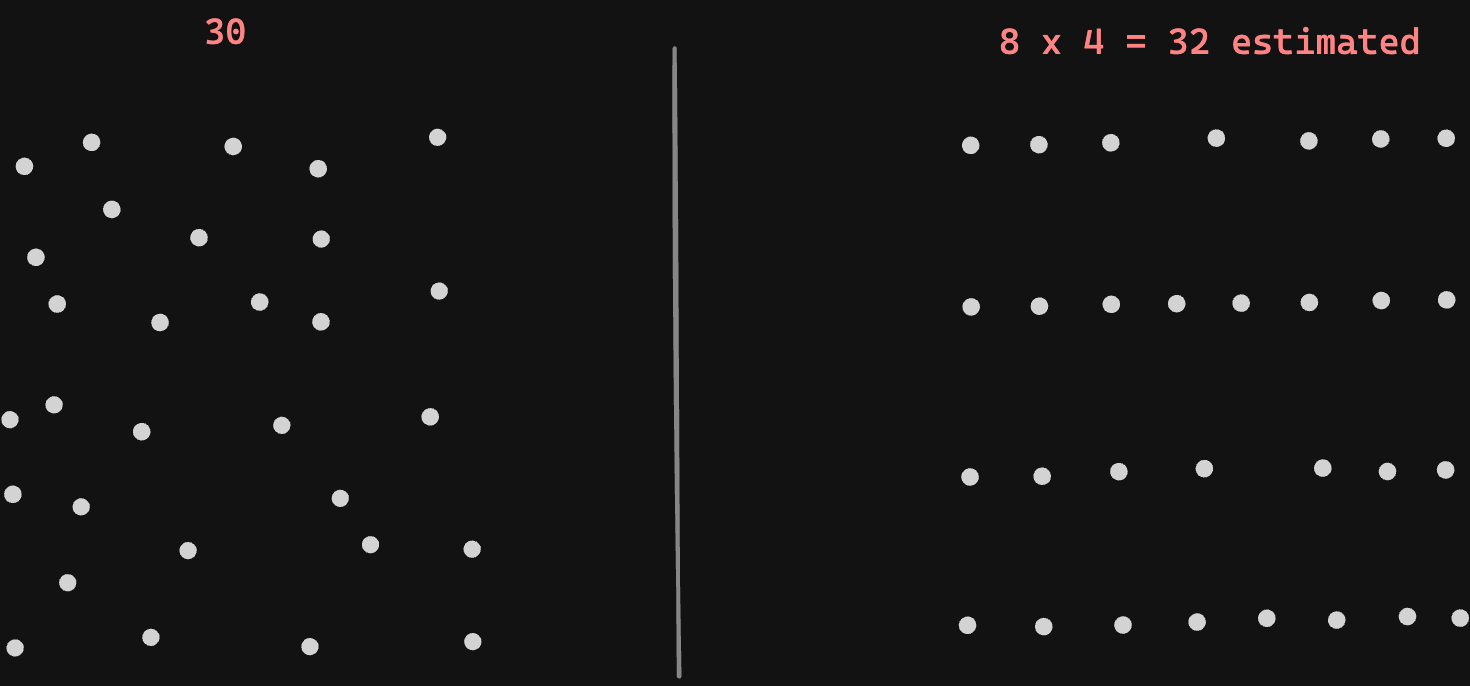
It’s sort of like this diagram above. If we arrange the dots in an organized manner, we can figure out an approx population count immediately by multiplying the number of rows and columns. As long as we know the number of rows and columns, we can arrive at the total count quickly, no matter how big the table gets. While when left unorganized (left) we would have to count each dot individually.
Hopefully you have a good conceptual idea of what a data sketch is. We can verify the data sketch with an actual code snippet.
import heapq as hq
import mmh3
import numpy as np

# ── Constants ─────────────────────────────────────────────────────────────────
RNG_SEED        = 25
MIN_EMPLOYEE_ID = 1
MAX_EMPLOYEE_ID = 4_000_000   # Walmart employee IDs in [1, 4M]
NUM_CHECKINS    = 2_000_000   # total check-ins today (duplicates expected)
K               = 1_000       # keep K lowest tags; error ≈ 1/√K ≈ 3.2%
TAG_SPACE       = 1 << 32     # tags in [1, ~4 billion] — must be >> unique employees
                              # to avoid collisions (1M tag space < 1.57M uniques = broken)

# ── Step 1: Simulate check-ins ────────────────────────────────────────────────
# 2M check-ins from employees with IDs in [1, 4M] — duplicates expected
rng      = np.random.default_rng(RNG_SEED)
checkins = rng.integers(MIN_EMPLOYEE_ID, MAX_EMPLOYEE_ID + 1, size=NUM_CHECKINS)

# ── Step 2: Build KMV sketch ──────────────────────────────────────────────────
# Each employee gets a deterministic integer tag in [1, TAG_SPACE] via hash.
# Same employee → same tag always, so duplicate check-ins are naturally skipped.
# Inspector keeps only the K lowest tags — O(K) memory regardless of stream size.
heap     = []    # max-heap (negated) — heap[0] = -(current K-th lowest tag)
heap_set = set() # mirrors heap for O(1) lookup — size stays ≤ K

for emp_id in checkins:
    tag = (mmh3.hash64(str(int(emp_id)), signed=False)[0] % TAG_SPACE) + 1

    if tag in heap_set:
        continue  # same tag already tracked (same employee checking in again)

    if len(heap) < K:
        hq.heappush(heap, -tag)
        heap_set.add(tag)
    elif tag < -heap[0]:          # smaller than current K-th tag — swap in
        evicted = -hq.heapreplace(heap, -tag)
        heap_set.discard(evicted)
        heap_set.add(tag)

# ── Step 3: Estimate unique headcount ─────────────────────────────────────────
# The K-th lowest tag sits at position K in the sorted uniform distribution.
# Average gap between tags = kth_tag / K
# Total unique employees  ≈ TAG_SPACE / gap = TAG_SPACE * K / kth_tag

kth_tag  = -heap[0]
gap      = kth_tag / K
estimate = TAG_SPACE / gap          # = TAG_SPACE * K / kth_tag

# ── Step 4: Verify ────────────────────────────────────────────────────────────
exact      = np.unique(checkins).size
error_rate = abs(estimate - exact) / exact

print(f"Tag space         : 1 to {TAG_SPACE:,}") # 1 to 4,294,967,296
print(f"K-th tag (K={K}) : {kth_tag:,}") # 2,779,252
print(f"Avg gap           : {gap:,.0f}") # 2,779
print(f"Estimate          : {estimate:,.0f}") # 1,545,368
print(f"Exact             : {exact:,}") # 1,574,043
print(f"Error             : {error_rate:.2%}  (expected ~{1/K**0.5:.2%})") # 1.82%  (expected ~3.16%)
Its all about probability
This can be confusing at first. How do we evenly distribute these numbers and ensure they are unique? The secret that this algo works is due to the magic inside the hash function (MurmurHash3). That is the crux of this solution. The hash function needs to be well tested and vetted to generate a uniform distribution of numbers on a large scale. The MurmurHash3 hash function in this case does that job. It distributes the hash output numbers equally across the space in complete isolation. And that happens due to the law of large numbers. We will dive deeper into that in another article, but to be brief, this algorithm ensures that every tag (hash) it generates has an equal chance of being placed anywhere on the scale. And with the probability laws in effect, these odds for these tags to get evenly distributed are massive (given the data points are large too).
Using this method, we can quickly estimate the counts for a metric. It comes in handy when we just need approximations and not absolute numbers. Especially on dashboards or reports.
These functions are available in most of the data storage platforms. In Spark you can use it to aggregate counts across clusters without shuffling data. In Postgres (postgresql-hll extension), you can use it to aggregate counts across days, weeks, months etc without manually going through the rows. So the next, time you require quick aggregations, consider using Data Sketches instead of count(). It’ll definitely save you a lot of compute cycles.
Hmm.. this is interesting. I wasn't aware of this. Thanks for this Lezwon